Arduino GPS Tracker
“As an Amazon Associates Program member, clicking on links may result in Maker Portal receiving a small commission that helps support future projects.”
The NEO-6 is a miniature GPS module designed by u-blox to receive updates from up to 22 satellite on 50 different channels that use trilateration to approximate fixed position of a receiver device every second (or less, for some modules). The particular module used in this tutorial, the NEO-6M, is capable of updating its position every second and communicates with an Arduino board using UART serial communication. The NEO-6M uses the National Marine Electronics Association (NMEA) protocol which provides temporal and geolocation information such as Greenwich Mean Time (GMT), latitude, longitude, altitude, and approximate course speed. The NEO-6M and Arduino board will also be paired with an SD module to create a portable logger that acts as a retrievable GPS tracker.
The GPS tracker will be fully contained and isolated from any external power or communication. In order to achieve this, we will need to use an SD card and LiPo battery. And after measuring the approximate current consumption of the whole Arduino GPS tracker at roughly 120mA-180mA, I decided to use an 850mAh battery, which yields 5-6 hours of tracking and saving to the SD card. The full parts list is given below with some affiliate and store links:
NEO-6M GPS Module - $15.00 [Our Store]
3.3V SD Module - $8.00 [Our Store]
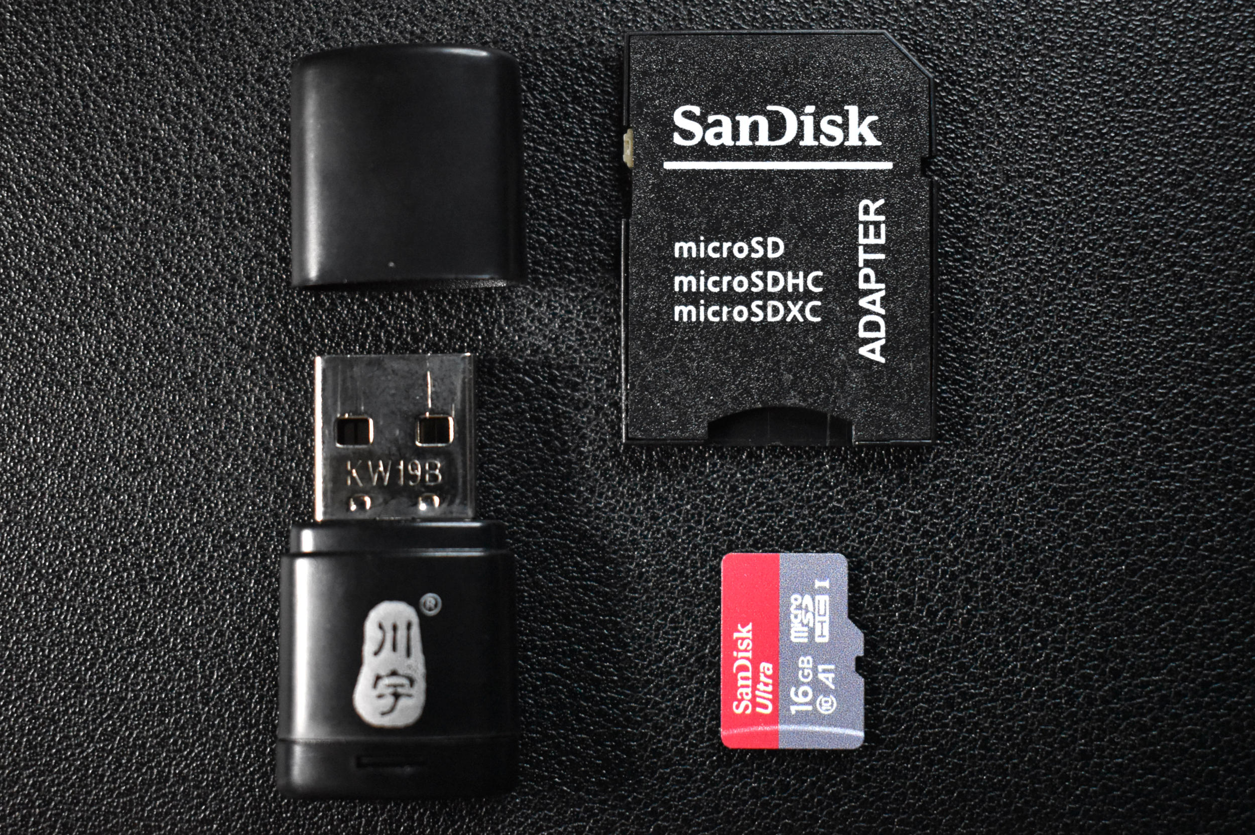
16GB Micro SD Card + USB Reader - $10.00 [Our Store]
850 mAh LiPo Battery - $18.99 (4 pcs + charger) [Amazon]
Arduino Uno - $11.00 [Our Store]
3.7V to 5.0V Buck Converter - $7.99 (2 pcs) [Amazon]
Jumper Wires - $6.98 (120 pcs) [Amazon]


The NEO-6 GPS Datasheet can be found here, where the specific workings of the module can be found. In short, the NEO-6M can update its fixed position roughly every second and can use anywhere between 3-22 satellites. The particular module communicates with the Arduino over UART (pins 5/6 are used here). The SD module uses SPI communication, with the chip select on pin 4. Pins 4/5/6 are therefore specifically determined in the code.
The full code is given below, followed by a description of the basic usage and output:
// Arduino code for NEO-6M + SD Card GPS Tracker
#include <SoftwareSerial.h>
#include <TinyGPS.h>
#include <SPI.h>
#include <SD.h>

const int chipSelect = 4;

TinyGPS gps; // GPS initialization
SoftwareSerial ss(6, 5); // pins for GPS (D5 -> GPS RX, D6 -> GPS TX)

static void smartdelay(unsigned long ms); // delay that also takes into account GPS
bool valid_date = false; // used for naming sd file
String filename = ""; // dummy placeholder, this will be updated later based on timestamp
String prev_date = ""; // ensuring the same data points aren't saved more than once

void setup() {
  Serial.begin(9600);

  if (!SD.begin(chipSelect)) {
    while (1); // do nothing if SD is not started
  }
  ss.begin(9600); // start GPS module
}

void loop() {

  float flat, flon;
  unsigned long age;
  String date_str;
  gps.f_get_position(&flat, &flon, &age);
  String datastring = "";
  date_str = find_date(gps,prev_date);
  prev_date = date_str;
  datastring+=date_str; datastring+=",";
  datastring+=String(flon,6); datastring+=",";
  datastring+=String(flat,6); datastring+=",";
  datastring+=String(gps.f_altitude(),6); datastring+=",";
  datastring+=String(gps.f_course(),2); datastring+=",";
  datastring+=String(gps.f_speed_kmph(),5);

  if (date_str=="NaN"){
  } else {
    if (valid_date==false){
      valid_date = true;
      filename = filenamer(gps);
      Serial.println(filename);
      File dataFile = SD.open(filename, FILE_WRITE);
      if (dataFile){
        dataFile.println("Date [mm/dd/yyyy HH:MM:SS],Longitude [deg],"
        "Latitude [deg],Altitude [m],Heading [deg],Speed [kmph]"); // alter based on data
        dataFile.close();
      } else {
        Serial.println("Issue with saving header");
      }
    } else {
      // open file, write to it, then close it again
      File dataFile = SD.open(filename, FILE_WRITE);
      if (dataFile) {
        Serial.print("data string: ");
        Serial.println(datastring);
        dataFile.println(datastring);
        dataFile.close();
      }
    }
  }

  smartdelay(1000);
}

static void smartdelay(unsigned long ms) {
  unsigned long start = millis();
  do
  {
    while (ss.available())
      gps.encode(ss.read());
  } while (millis() - start < ms);
}

String find_date(TinyGPS &gps,String prev_date) {
  int year;
  byte month, day, hour, minute, second, hundredths;
  unsigned long age;
  String date_str = "";
  gps.crack_datetime(&year, &month, &day, &hour, &minute, &second, &hundredths, &age);
  if (age == TinyGPS::GPS_INVALID_AGE)
    date_str = "NaN";
  else
  {
    int byte_size = 19;
    char chars[byte_size];
    sprintf(chars, "%02d/%02d/%02d %02d:%02d:%02d",
          month,day, year, hour, minute, second);
    for (int ii=0;ii<=byte_size-1;ii++){
      date_str+=String(chars[ii]);
    }

  }
  if (date_str==prev_date){
    return "NaN";
  }
  return date_str;
}

String filenamer(TinyGPS &gps) {
  int year;
  byte month, day, hour, minute, second, hundredths;
  unsigned long age;
  gps.crack_datetime(&year, &month, &day, &hour, &minute, &second, &hundredths, &age);
  String filename = "";
  int byte_size = 8;
  char chars[byte_size];
  sprintf(chars, "%02d%02d%02d%02d",
        day, hour, minute, second);
  for (int ii=0;ii<=byte_size-1;ii++){
    filename+=String(chars[ii]);
  }
  return filename+".csv";
}
The code follows the outline specified below:
Plug in LiPo battery
Arduino checks that both the NEO-6M and SD module are wired and started correctly
If a valid GPS signal is received, create a .csv file based on the date in the format: “ddHHMMSS.csv” - where dd is day, HHMMSS are hour, minute, and second; respectively.
The GPS data will be logged onto the .csv file in the following column format (with headers):
Date [mm/dd/YYY HH:MM:SS], Longitude [degrees], Latitude [degrees], Altitude [meters], Heading [degrees], Speed [km/hour]
-Note on GPS connection speed-
The NEO-6M needs 10-60s to connect to at least 3 satellites. The NEO--6M should be blinking its light if it is appropriately communicating with satellites. If it takes longer than a minute, unplug and restart the GPS module. Once the GPS's light is connected, it will stay connected (unless there is interference with metal or structures).

A Simple Cardboard Box Housing for the GPS Tracker
QGIS is a geographic information system (GIS) tool used by geographers, statisticians, and engineers interested in geographic-related visualization. QGIS is an open-source tool and fairly easy to use. Click the logo below to go directly to the QGIS download page. I recommend downloading the stable release. I will be using QGIS 2.8.9 (2016), but 3.x versions have been made and the newer downloads should work just the same.
The user should download a map base, in my case I’m using Bing’s road map. You can use Google or other basemaps. You can insert the basemap by:
Click “Web”
“Web -> OpenLayers Plugin -> Bing Maps -> Bing Road”
If there is no OpenLayers plugin, it will need to be downloaded by following the process outlined at https://support.dronesmadeeasy.com/hc/en-us/articles/115003641026-QGIS-Installing-Google-Maps-Plugin essentially it follows:
Click “Plugins”
Click “Manage and Install Plugins …”
Type in “openlayers”
Click on “OpenLayers Plugin”
Install Plugin
Follow the process above after install
For my particular case, I walked around New York City and mapped the route using various basemaps (Bing Maps, OpenStreetMap, Wikipedia Labeled Layer). Below is a sample mapping where I walked around the campus at the City College of New York, and the data points from the GPS sensor match nearly exactly with the route taken. When walking near some larger buildings, the GPS lags or jumps around, which is expected as it is likely that the satellites are having trouble communicating with the sensor through or around the taller masses.
Below is the GPS route atop the Bing aerial street map, which closely resembles a satellite image of the surface:
The OpenStreetMap of the same route is shown below:
Wikipedia also has a labeled layer, similar to the OpenStreetMap layer:
Here is another route atop the OpenStreetMap:
QGIS is a powerful tool for static visualization, but if we really want to dig into the GPS data, Python is a better fit for many reasons. I wanted to clean up the data, and I find it much easier to get rid of erroneous points in Python rather than QGIS. Time series analysis is also very difficult in GIS software, so I will do that in Python. Lastly, I will create some animations that I wouldn’t even know how to broach with the QGIS software.
Below are two mappings of the routes above with different basemaps, both plotted in Python with the Basemap toolkit:
The code to replicate the plots above is given below:
# Python code for plotting GPS data from Arduino
from mpl_toolkits.basemap import Basemap
import numpy as np
import matplotlib.pyplot as plt
import csv,os

# find files in directory that are .csv
csv_files = [file for file in os.listdir('.') if file.lower().endswith('.csv')]

# preallocate variables and loop through given file
t_vec,lons,lats,alts,headings,speeds = [],[],[],[],[],[]
header = []
with open(csv_files[0],newline='') as csvfile:
    reader = csv.reader(csvfile,delimiter=',')
    for row in reader:
        if header == []:
            header = row # header with variable names and units
            continue
        t_vec.append(row[0])
        lons.append(float(row[1]))
        lats.append(float(row[2]))
        alts.append(float(row[3]))
        headings.append(float(row[4]))
        speeds.append(float(row[5]))

# plotting the lat/lon points atop map
fig = plt.subplots(figsize=(14,8))
x_zoom = 0.004
y_zoom = 0.0015
bmap = Basemap(llcrnrlon=np.min(lons)-x_zoom,llcrnrlat=np.min(lats)-y_zoom,
              urcrnrlon=np.max(lons)+x_zoom,urcrnrlat=np.max(lats)+y_zoom, epsg=4326)

bmap.scatter(lons,lats,color='r',edgecolor='k') # plot lat/lon points

# basemap behind scatter points

# the best basemap services:
##map_service = 'World_Imagery' # high-resolution satellite map
map_service = 'World_Topo_Map' # higher resolution map similar to google maps

# other basemaps
##map_service = 'ESRI_StreetMap_World_2D' # similar to 'World_Topo_Map' but fewer definition
##map_service = 'USA_Topo_Maps' # topographic map (similar to road maps)
##map_service = 'NatGeo_World_Map' # low-resolution map with some labels
##map_service = 'World_Street_Map' # street map at higher resolution with labels
##map_service = 'World_Terrain_Base' # terrain map (low resolution, non-urban, no streets)
##map_service = 'ESRI_Imagery_World_2D' # lower resolution satellite image map

bmap.arcgisimage(service=map_service, xpixels = 1000, verbose= True) #basemap plot

plt.tight_layout(pad=0.0)
plt.show()
Using Heading and Speed:
Next, I’ll be using the heading and speed to create a quiver plot that can represent the speed and direction of travel on the map. The way we do this is by looking at the geometry of the heading outputted by the GPS. The NEO-6M outputs heading information which in short calculates the heading based on consecutive points. A typical compass uses true north as 0° and counts clockwise movements as positive changes in heading.
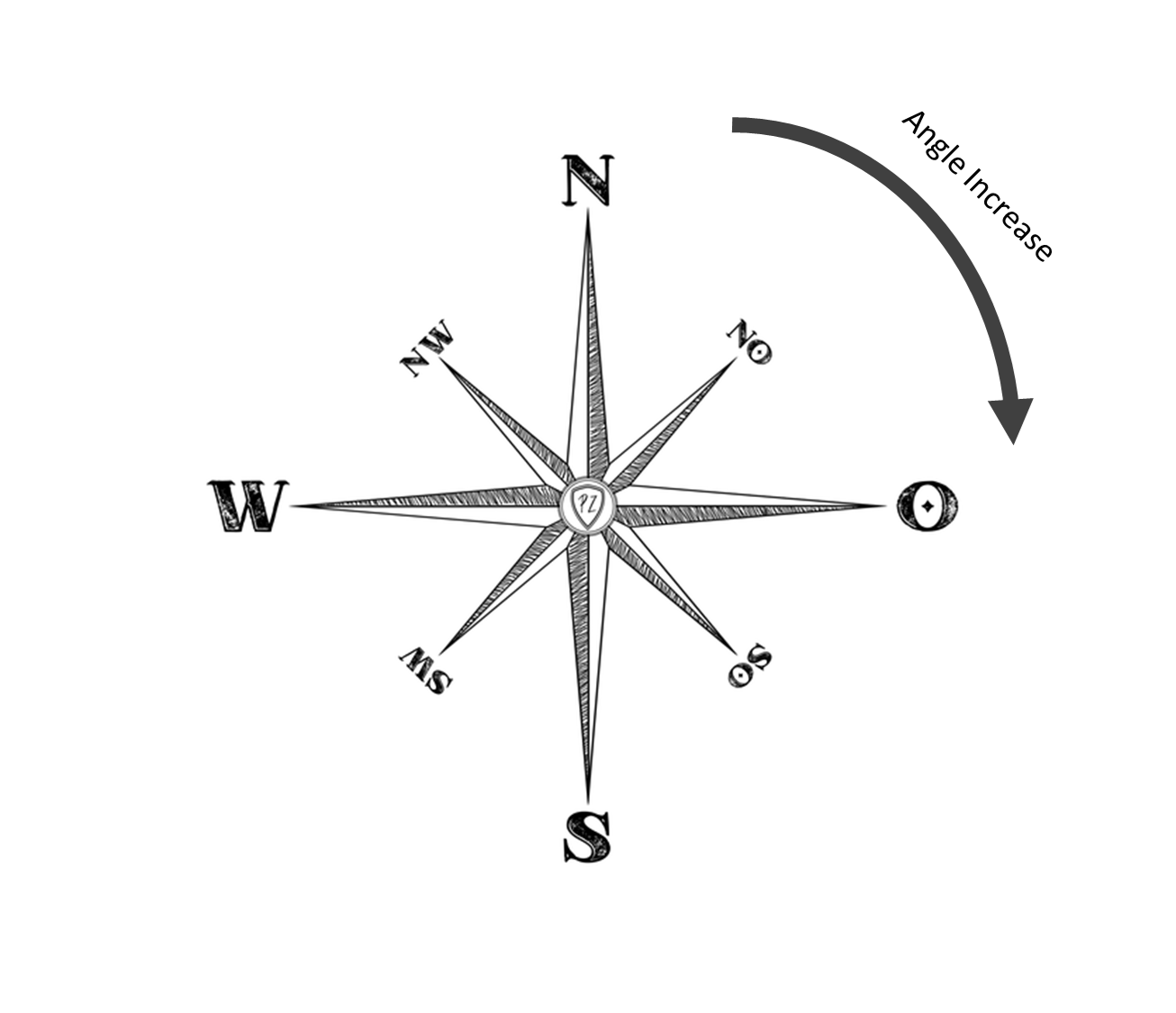
An increase in GPS heading is associated with a clockwise rotation with respect to true north
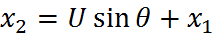
We can derive a relationship between the heading, speed, and latitude and longitude points on the surface of the earth. Invoking geometry:


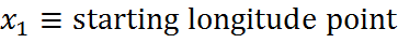


Calculating each quiver point

Plotting the quiver points using Python, we get the following mapped result:
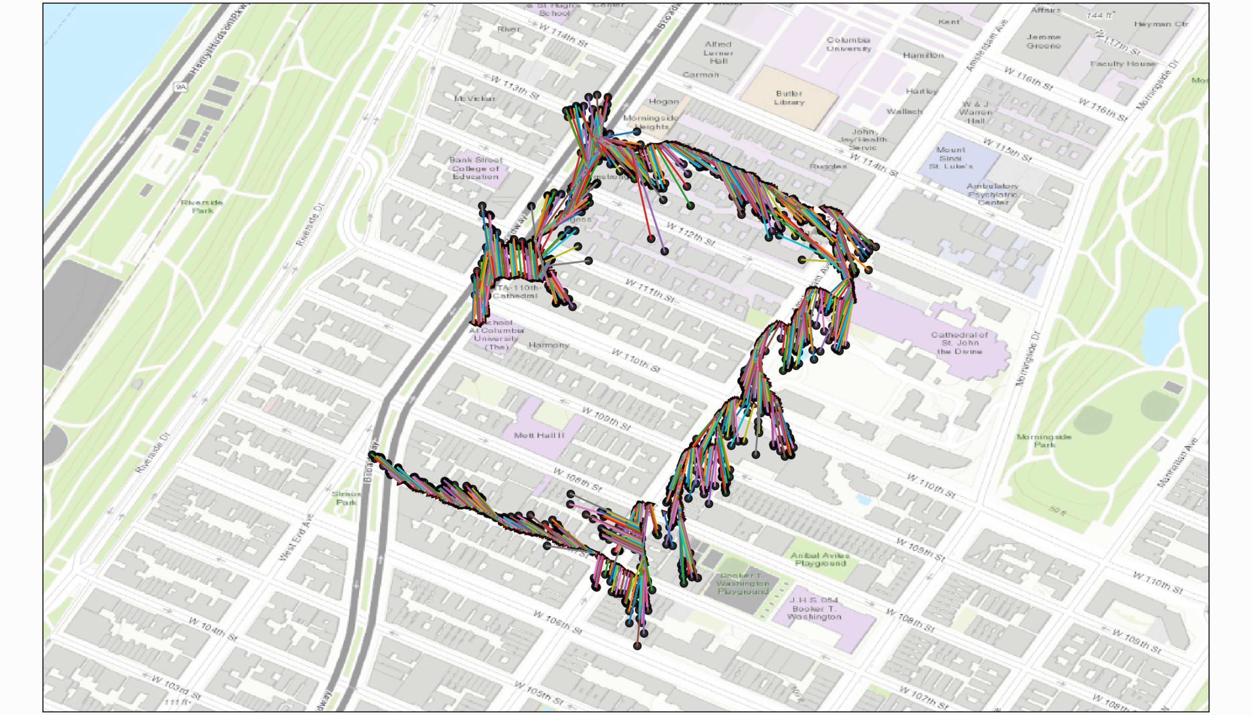
The plot above shows the rough direction of travel. To start, the upper-left portion of the GPS data is moving north, and the right-hand data is moving south. This is the trend that was followed during acquisition. The quivers can be helpful for determining direction and speed of travel, which we can see here is fairly accurate, though a bit noisy.
The other route is shown below, which started in the upper-right and followed a clockwise travel direction - which is mostly captured with the quiver plot, especially on the left-hand side of the route (where there’s less interference from buildings).

The full quiver code is also given below:
# Python code for plotting GPS directional quivers
from mpl_toolkits.basemap import Basemap
import numpy as np
import matplotlib.pyplot as plt
import csv,os

# find files in directory that are .csv
csv_files = [file for file in os.listdir('.') if file.lower().endswith('.csv')]

# preallocate variables and loop through given file
t_vec,lons,lats,alts,headings,speeds = np.array([]),np.array([]),np.array([]),\
                                       np.array([]),np.array([]),np.array([])
header = []
with open(csv_files[3],newline='') as csvfile:
    reader = csv.reader(csvfile,delimiter=',')
    for row in reader:
        if header == []:
            header = row # header with variable names and units
            continue
        t_vec = np.append(t_vec,row[0])
        lons = np.append(lons,float(row[1]))
        lats = np.append(lats,float(row[2]))
        alts = np.append(alts,float(row[3]))
        headings = np.append(headings,float(row[4]))
        speeds = np.append(speeds,float(row[5]))

# plotting the lat/lon points atop map and calculating quivers
fig = plt.subplots(figsize=(14,8))
x_zoom = 0.004
y_zoom = 0.0015
bmap = Basemap(llcrnrlon=np.min(lons)-x_zoom,llcrnrlat=np.min(lats)-y_zoom,
              urcrnrlon=np.max(lons)+x_zoom,urcrnrlat=np.max(lats)+y_zoom, epsg=4326)

speeds = 10.0*speeds*((np.mean(np.abs(np.diff(lats)))+np.mean(np.abs(np.diff(lons))))/2.0)
for ii in range(0,len(lons)):
    lon_2 = (speeds[ii]*np.sin(headings[ii]*(np.pi/180.0)))+lons[ii] # quiver calcs
    lat_2 = (speeds[ii]*np.cos(headings[ii]*(np.pi/180.0)))+lats[ii] # quiver calcs

    bmap.plot([lons[ii],lon_2],[lats[ii],lat_2]) # drawing lines
    bmap.scatter(lons[ii],lats[ii],color='r',marker=(3,0,-headings[ii]+90),
                 edgecolor='k',alpha=0.8) # drawing and rotating triangles at GPS point
    bmap.scatter(lon_2,lat_2,color='k',marker='o',
                 edgecolor='k',alpha=0.8) # drawing a circle at the end of quiver

# basemap behind scatter points

# the best basemap services:
##map_service = 'World_Imagery' # high-resolution satellite map
map_service = 'World_Topo_Map' # higher resolution map similar to google maps
bmap.arcgisimage(service=map_service, xpixels = 1000, verbose= True) #basemap plot
plt.tight_layout(pad=0.0)
plt.show()
Mapping Over Time:
For the time series map, I’ll just be plotting point-by-point to see how and at which point each GPS point was set (at some interval, which I set depending on the size of the route). Below is an animation of the GPS route, which was created using Python and a .gif creator algorithm. The route roughly follows the trajectory laid out by the quiver plot.
The code to replicate this is also given below:
# Python code for real-time plotting of Arduino GPS data
from mpl_toolkits.basemap import Basemap
import numpy as np
import matplotlib.pyplot as plt
import csv,os

# find files in directory that are .csv
csv_files = [file for file in os.listdir('.') if file.lower().endswith('.csv')]

# preallocate variables and loop through given file
t_vec,lons,lats,alts,headings,speeds = np.array([]),np.array([]),np.array([]),\
                                       np.array([]),np.array([]),np.array([])
header = []
with open(csv_files[0],newline='') as csvfile:
    reader = csv.reader(csvfile,delimiter=',')
    for row in reader:
        if header == []:
            header = row # header with variable names and units
            continue
        t_vec = np.append(t_vec,row[0])
        lons = np.append(lons,float(row[1]))
        lats = np.append(lats,float(row[2]))
        alts = np.append(alts,float(row[3]))
        headings = np.append(headings,float(row[4]))
        speeds = np.append(speeds,float(row[5]))

# plotting the lat/lon points atop map and calculating quivers
fig = plt.subplots(figsize=(14,8),facecolor=[252.0/255.0,252.0/255.0,252.0/255.0])
plt.ion()
x_zoom = 0.004
y_zoom = 0.0015
bmap = Basemap(llcrnrlon=np.min(lons)-x_zoom,llcrnrlat=np.min(lats)-y_zoom,
              urcrnrlon=np.max(lons)+x_zoom,urcrnrlat=np.max(lats)+y_zoom, epsg=4326)
# the best basemap services:
##map_service = 'World_Imagery' # high-resolution satellite map
map_service = 'World_Topo_Map' # higher resolution map similar to google maps
bmap.arcgisimage(service=map_service, xpixels = 1000, verbose= True) #basemap plot

for ii in np.arange(0,len(lons),int(len(lons)/50)):
    bmap.scatter(lons[ii],lats[ii],color='r',marker='o',edgecolor='k',alpha=0.8)
    plt.pause(0.001)

plt.tight_layout(pad=0.0)
plt.show()
The goal of this tutorial was to develop a portable and self-contained GPS tracker. With Arduino, I paired the NEO-6M GPS module and SD card to act as the GPS logging system. Using the system, 1Hz update rates from the GPS system was achievable. I analyzed two routes in QGIS and Python, demonstrating the accuracy and ability to analyze the data produced by the Arduino GPS tracker. I also introduced some methods for visualizing in Python that were more involved, such as quiver plots and time-related plots. This tutorial was meant to demonstrate the capability of the NEO-6M GPS module and the power of Python for analysis of geographic data.
More in Python, Arduino, and GIS: